Distances in Machine Learning (Pt. 3 – Model Distances)

We’ve seen how distances can be used in machine learning and data mining for different types of data, but we don’t only look at data in these areas. Remember in part one we looked at traditional, numerical distances that match our intuitions about distances and in part two we look at ways to measure the distance between strings. But what about mathematical models?

Models are everywhere in machine learning and data mining. We produce them to summarize data and to make predictions about the environment. But what if we get different models from two different data sets, or at two points in time? How different is too different and when can we say that something has changed?

To answer these questions we can turn to a set of mathematical tools that I will call model distances.

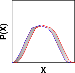
So many times in machine learning, we end up producing models that are represented as probability distributions. Of course we might have many models, and as always we might want to know “how far apart” these models are. The usual reason to build models is to make predictions, so what if we saw that the distance between two models is the distance between their predictions?

The Hellinger distance does exactly this with two probability distributions. This distance is calculated as an integral across the whole domain of two probability distributions. If our probability distributions are named \(f(x)\) and \(g(x)\) then we calculate the Hellinger distance between them as: $$H^2(f,g) = \frac{1}{2} \int \left(\sqrt(f(x)) – \sqrt(g(x))\right)^2 \, dx$$

Looking closely at this expression we see that any divergence between the values of \(f\) and \(g\) increases the distance between the distributions; the larger the divergence the larger the increase in distance. We can also see that identical values have no effect on the distance between the distributions and that we can never reduce the distance that has already accumulated.

There are specific forms of the Hellinger distance for simple probability distributions, such as normal distributions, that allow you to simplify your calculations by skipping the integral–great for programming implementations!

The variation of information is a measure that comes from information theory. As an aside, I think that information theory is an amazingly powerful area of math for both machine learning and data mining; I have never regretted learning more.

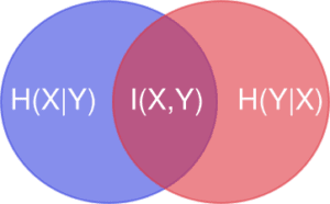
But back to our point of interest, the variation of information between two partitions measures how much information (in the mathematical sense) is shared between the two partitions of a set. If knowing about partition \(X\) tells you everything you need to know about partition \(Y\) (and vice versa), then the partitions are close to each other. If instead knowledge of \(X\) tells you next to nothing about \(Y\), then the partitions are far apart.

If we know the conditional entropies of \(X\) and \(Y\) given the other as well as their mutual information, then we can calculate that variation of information between \(X\) and \(Y\) as $$V(X,Y) = H(X) + H(Y) – 2I(X,Y)$$ or as $$V(X,Y) = H(X|Y) + H(Y|X).$$

Similar to the variation of information, the Tversky index comes from the fields of psychology and decision-making. Here we model the problem as one of comparing an object’s features with a prototype’s features.

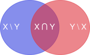
Here we model our underlying objects as sets of features. For example, an apple might have the features \(\{red,sweet,round\}\) while a car might have the features \(\{large,blue,affordable\}\). If \(X\) is the set of features for the object and \(Y\) is the set of features for the prototype, then the Tversky index between them is $$S(X,Y) = \frac{|X \cap Y|}{|X \cap Y| + \alpha |X \setminus Y| + \beta |Y \setminus X|}.$$

The Tversky index allows different weights to be assigned to features in the object and the prototype to model their relative importance. If \(\alpha\) is large then we want our object to only have prototypical features  and if \(\beta\) is large then we want our object to have all of the prototypical features.

Although we notice that the Tversky index is not a true distance function because it is not symmetric, this is actually a feature when it comes to explaining some of the idiosyncrasies in human decision-making. As Amos Tversky explained in his original paper, this asymmetry accounts for findings like:

1. We would say that an ellipse is like a circle more than we would say that a circle is like an ellipse; and
2. In writing, similes often only work in one direction: “his anger burned like the sun” makes much more sense than “the sun burned like his anger.”

If our goal for data mining is to understand individual preferences, then keeping this asymmetry in mind is key.

So now we’ve covered some ways that we can formalize the distance between two models. These can be useful whenever we produce models in machine learning and data mining. Which is always.

The main reason why we’d want to know how far apart to models are is to know if there is a practical differences between the models:

1. I used the Hellinger distance to model the distance between two concepts in my Mixture Model Generator (see our paper for the full description). If a data set’s underlying concept changes over time, we should verify whether our original models are still useful;
2. The variation of information can be used to compare different clusterings and therefore different clustering algorithms. In a similar vein, I developed a cluster distance function to measure the distance between two individual clusters within a clustering; and
3. Even though it’s not a true distance, the Tversky index illuminates some of the foibles in how humans compare objects.